FP8 Inference: What It Means for Your API Bill

FP8 inference can reduce the memory and computation required to serve a large language model. That does not mean every FP8 model comes with a lower API price. Your final bill still reflects the selected model, input length, output length, cache usage, retries, and task success rate. To estimate the real cost, developers need to look beyond the precision label.

What Is FP8 Inference?

FP8 inference uses eight-bit floating-point formats for selected model weights, activations, or operations during model serving.

Unlike INT8, FP8 retains a floating-point structure with a sign, exponent, and mantissa. This allows it to represent values across a wider numerical range than a standard eight-bit integer format.

Two common FP8 formats are:

· E4M3: one sign bit, four exponent bits, and three mantissa bits

· E5M2: one sign bit, five exponent bits, and two mantissa bits

E4M3 provides more mantissa precision within a smaller range. E5M2 provides a much wider range but stores values less precisely. Scaling methods help map model values into the range that each format can represent.

The term “FP8 model” does not always describe the same implementation. It may refer to:

· FP8 weights with higher-precision activations

· FP8 weights and activations, often described as W8A8

· An FP16 or BF16 checkpoint converted during deployment

· A mixed-precision system that keeps sensitive operations at higher precision

· Different FP8 formats or scaling methods across individual tensors

FP8 inference therefore does not mean every calculation runs in eight-bit precision. The actual configuration depends on the model checkpoint, serving framework, hardware support, calibration method, and inference kernels.

FP8 vs. FP16 vs. BF16

FP8, FP16, and BF16 all represent floating-point values, but they divide their available bits differently.

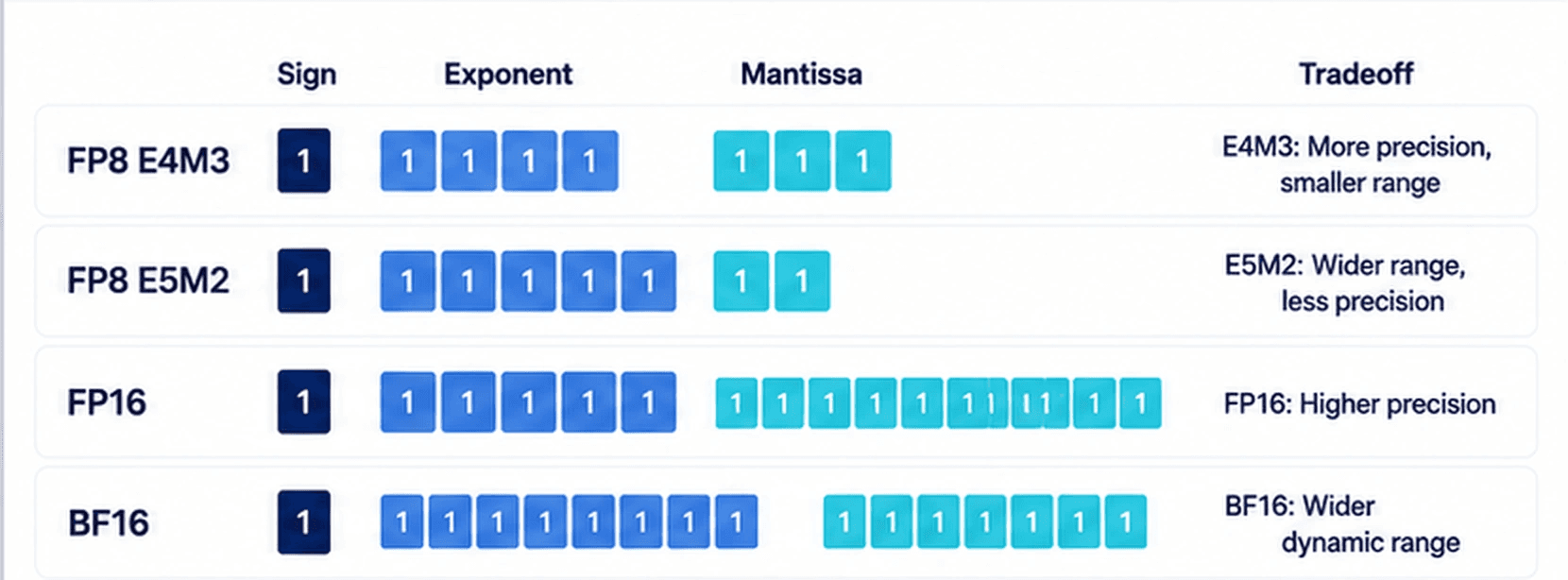
BF16 uses the same number of exponent bits as FP32, giving it a wider dynamic range than FP16. FP16 uses more mantissa bits, so it represents values more precisely within its available range. The better format depends on the numerical behavior of the workload rather than a universal accuracy ranking.

An FP8 value requires half the raw storage of an FP16 or BF16 value. However, a complete inference service also needs memory for:

· KV cache data

· Temporary tensors

· Scaling factors

· Request state

· Higher-precision accumulations

· MoE routing data

· Framework and communication overhead

FP8 can substantially reduce model-weight memory requirements, but total GPU memory does not automatically fall by exactly 50%.

Why Precision Can Affect API Cost

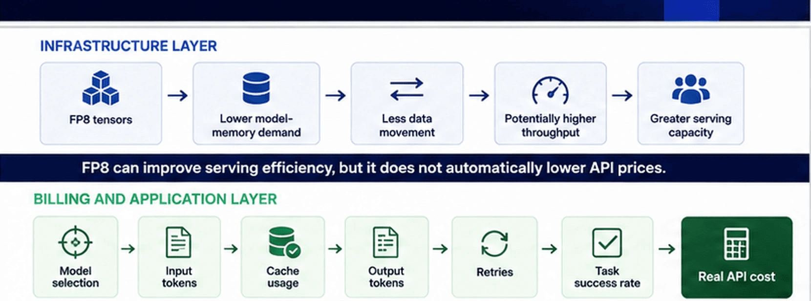
Precision can influence LLM inference cost through memory use, data movement, compute throughput, and serving capacity.

Lower Model Memory Demand

Model weights occupy a large share of GPU memory. Reducing their precision may allow a model to fit on fewer accelerators or leave more memory available for active requests.

That additional capacity may support:

· Larger batches

· More concurrent requests

· Longer contexts

· A larger KV cache

· Less model partitioning across GPUs

These improvements can increase the number of tokens served by the same hardware resources.

Less Data Movement

LLM inference repeatedly moves weights and other tensors between GPU memory and compute units. Smaller tensors reduce the amount of data transferred during supported operations.

This is particularly relevant during token generation, where memory bandwidth can become a limiting factor. Reducing the number of bytes moved per operation may improve throughput even when the underlying model architecture remains unchanged.

Higher Compute Throughput

Modern accelerators can execute FP8 matrix operations through dedicated hardware support. When the model, GPU, kernels, and inference framework use a compatible FP8 configuration, the system may process more operations in the same period.

For supported W8A8 configurations, vLLM documents a twofold reduction in model memory requirements and up to a 1.6-fold throughput improvement. These figures describe specific hardware and software conditions, not a guaranteed result for every model or workload.

Lower-precision tensors alone are not enough. Batching, memory management, kernel design, request scheduling, and multi-GPU communication determine whether theoretical FP8 efficiency becomes measurable production performance.

SiliconFlow combines a self-developed inference engine with end-to-end optimization across high-performance GPU infrastructure. Developers can access these optimized deployments through Serverless APIs or choose dedicated and custom options for workloads that require greater capacity control. The unified, OpenAI-compatible API also reduces the integration work required to test models under the same application logic.

Does FP8 Always Make an LLM API Cheaper?

No. FP8 can lower part of the infrastructure cost of serving a model, but public API pricing reflects far more than numerical precision.

Other pricing factors include:

· Model architecture and size

· Activated parameters per token

· Context and KV cache requirements

· Average output speed

· GPU utilization

· Cross-device communication

· Capacity and reliability requirements

· Model demand

· Platform pricing strategy

On SiliconFlow, Serverless model pages present input and output rates per million tokens. Some models also have a separate cache-read rate. The developer pays the published rates for the selected deployment rather than receiving a separate FP8 discount.

The following two models show why deployment precision cannot predict the final price by itself:

Prices were checked on July 15, 2026 and may change. The current model pages also show that Qwen3.6-27B has 27 billion total and activated parameters, while DeepSeek-V4-Flash activates 13 billion parameters per token.

Both deployments are marked FP8, yet their token prices differ significantly. They also have different architectures, capabilities, context limits, and expected workloads.

A lower token rate does not always produce a lower cost per completed task. A model may become more expensive in practice when it:

· Generates unnecessarily long responses

· Requires repeated attempts

· Produces invalid structured output

· Fails tool calls

· Needs additional verification

· Triggers a fallback model

· Completes fewer tasks successfully

The useful question is not simply whether a model uses FP8. It is how much the full workflow costs after quality, output length, retries, and reliability are included.

How FP8 Connects to MoE Models

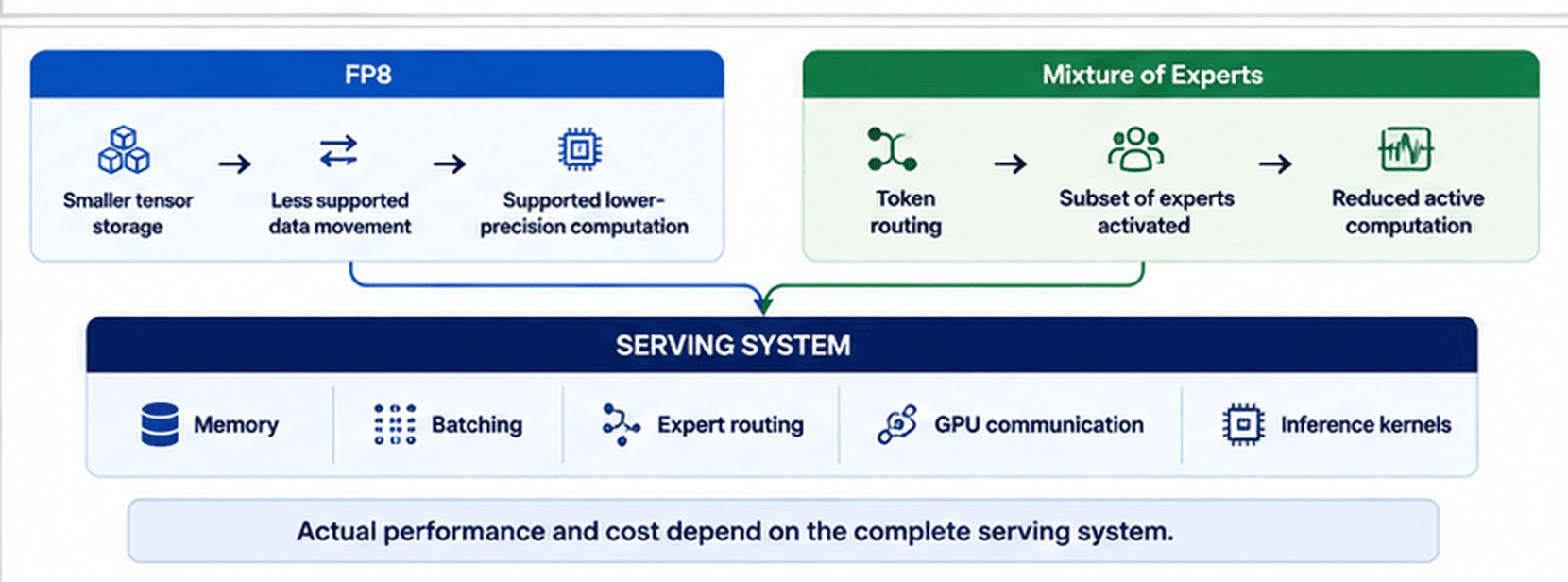
FP8 and Mixture-of-Experts address different parts of inference efficiency.

FP8 changes how selected values are stored and processed. MoE changes how model parameters are activated for each token.

A dense model normally uses all its parameters during each forward pass. An MoE model contains multiple expert networks but routes each token to a smaller group of experts.

DeepSeek-V3 provides a clear example. It contains 671 billion total parameters but activates approximately 37 billion for each token.

This creates two separate efficiency layers:

1. MoE reduces the number of parameters involved in each token’s computation.

2. FP8 reduces the storage and supported computation required for many of those tensors.

DeepSeek-V4-Flash further illustrates the relationship. The official model card identifies it as an MoE model with 284 billion total parameters and 13 billion activated parameters. Its released Instruct checkpoint combines FP4 expert parameters with FP8 for most other parameters, while the current SiliconFlow deployment is marked FP8 on the model page.

An MoE model is not equivalent to a dense model with the same number of activated parameters. The serving system must still manage:

The complete set of expert weights

· Expert routing

· Load balancing

· Expert parallelism

· Communication between GPUs

· Uneven expert demand across a batch

MoE reduces active computation, while FP8 can reduce memory and compute requirements. The final result depends on how well the architecture, hardware, and serving system operate together.

What Developers Should Check Before Choosing a Model

Precision is only one part of a production model evaluation. Developers should compare models using consistent prompts, parameters, datasets, and success criteria.

Each SiliconFlow model page provides deployment information such as architecture, precision, context length, pricing, and supported functionality. Developers can use these fields to create an initial shortlist before running application-specific tests.

The platform currently provides access to more than 200 optimized language and multimodal models through a unified API. This makes it practical to test several candidates without rebuilding the entire integration for every model. Serverless access supports usage-based experimentation, while dedicated and custom deployment options suit workloads that need more predictable capacity or infrastructure control.

A useful benchmark should measure more than accuracy. Record:

· Average input tokens

· Average output tokens

· Task success rate

· Retry rate

· Tool-call success

· Response latency

· Cost per request

· Cost per successful task

This approach shows whether a lower-priced model actually reduces the cost of running the application.

How to Estimate Your Real API Bill

Begin with the current rates for the selected model.

For a model with separate input and output prices:

Input cost =input tokens ÷ 1,000,000 × input rate

Output cost =output tokens ÷ 1,000,000 × output rate

Total token cost =input cost + output cost

For a model with a separate cache-read rate:

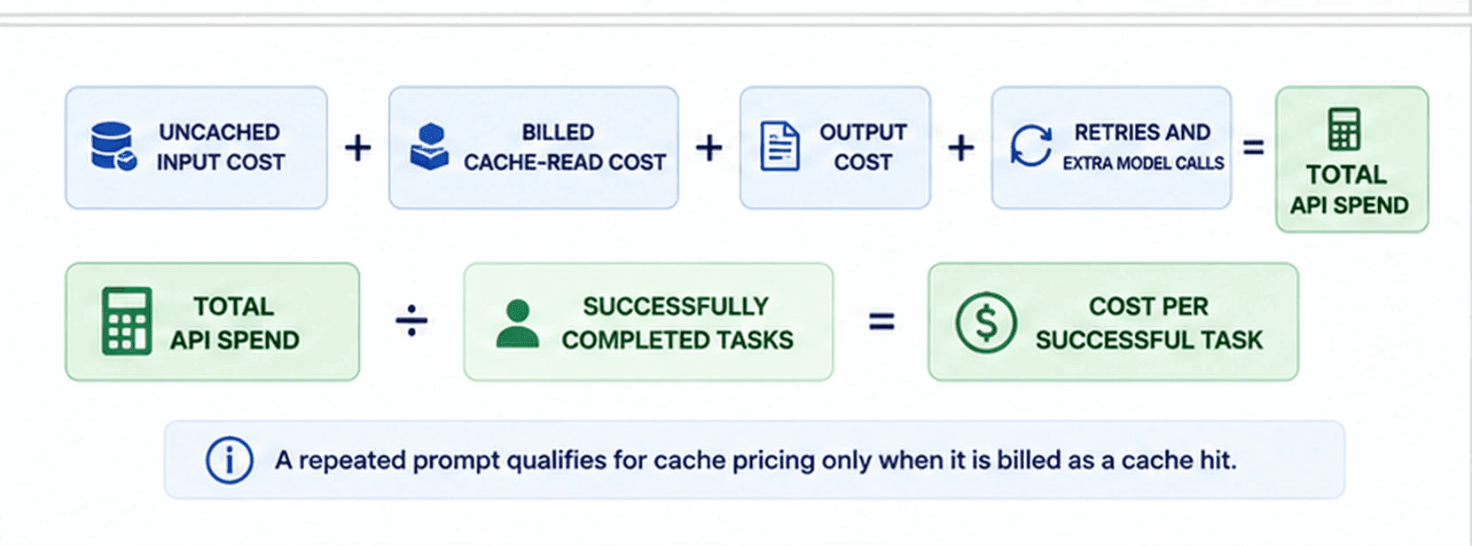
Total token cost =uncached input cost+ billed cache-read cost+ output cost

This produces a nominal request cost. A production estimate needs several additional steps.

Record Actual Token Usage

The SiliconFlow Chat Completions response includes prompt_tokens, completion_tokens, and total_tokens. Use these values instead of estimating token volume from characters or words.

Treat Cache Savings Conservatively

A repeated prompt does not necessarily qualify for the lower cache-read rate. Apply that rate only to input that is actually billed as a cache hit.

When cache-hit data is unavailable, estimate repeated input at the standard input rate. This prevents expected savings from being overstated.

Include Every Billable Model Call

One user action may trigger several requests. Agent workflows can plan, call tools, correct errors, verify results, and produce a final response.

Include costs from:

· Billable retries

· Tool-call correction loops

· Structured-output repairs

· Verification requests

· Regenerated responses

· Fallback model calls

These additional requests can matter more than a small difference in the listed input rate.

Measure Cost per Successful Task

The most useful production metric is often:

Cost per successful task =

total API spend ÷ successfully completed tasks

For example, one model may have a lower output price but require frequent retries. Another may cost more per token but complete the same task correctly on the first attempt.

The second model can still have the lower real cost.

Control Output Length

Output prices can differ substantially from input prices. A model that generates long responses may create a larger bill even when its input rate is low.

Use:

· Clear response requirements

· Suitable output limits

· Defined JSON fields

· Explicit stop conditions

· Controlled agent iteration counts

· Focused retrieval context

These settings reduce unnecessary tokens without relying on precision changes.

Test a Representative Workload

Evaluate models using real application inputs, including short, long, ambiguous, and failure-prone cases.

Because the API is OpenAI-compatible and unified across supported models, developers can change the model identifier while retaining much of the surrounding application logic. This makes it easier to compare token usage, quality, latency, and reliability under similar conditions.

FP8 Inference and API Cost FAQs

Q1. Does FP8 Inference Automatically Reduce API Prices?

No. FP8 may improve serving efficiency, but API rates also reflect model architecture, hardware utilization, capacity, performance, and platform pricing.

Q2. Is FP8 Less Accurate Than BF16?

It can be. FP8 represents fewer numerical values, so scaling, calibration, mixed-precision handling, and model design affect accuracy. Test each deployment with your own workload.

Q3. Can Developers Select FP8 in Each API Request?

Not in the standard Serverless workflow. Developers select an available model deployment rather than changing its serving precision for every request.

Q4. Are FP8 MoE Models Always the Cheapest Option?

No. MoE reduces active computation, while FP8 reduces supported tensor storage and computation. Routing, communication, output length, and token prices still affect the bill.

Q5. What Is the Best Metric for Comparing LLM Inference Cost?

Cost per successful task is more useful than token price alone. It includes output length, retries, tool loops, reliability, and the number of calls needed to complete real work.